Fixing Random, part 34

Last time on FAIC we implemented a better technique for estimating the expected value of a function f applied to samples from a distribution p:

• Compute the total area (including negative areas) under the function x => f(x) * p.Weight(x)
• Compute the total area under x => p.Weight(x)
  • This is 1.0 for a normalized PDF, or the normalizing constant of a non-normalized PDF; if we already know it, we don't have to compute it.
• The quotient of these areas is the expected value

Essentially our technique was to use quadrature to get an approximate numerical solution to an integral calculus problem.

However, we also noted that it seems like there might still be room for improvement, in two main areas:

• This technique only works when we have a good bound on the support of the distribution; for my contrived example I chose a "profit function" and a distribution where I said that I was only interested in the region from 0.0 to 1.0.
• Our initial intuition that implementing an estimate of "average of many samples" by, you know, averaging many samples, seems like it was on the right track; can we get back there?

In this episode I'm going to stick to the restriction to distributions with support over 0.0 to 1.0 for pedagogic reasons, but our aim is to find a technique that gets us back to sampling over arbitrary distributions.

The argument that I'm going to make here (several times!) is: two things that are both equal to the same third thing are also equal to each other.

Recall that we arrived at our quadrature implementation by estimating that our continuous distribution's expected value is close to the expected value of a very similar discrete distribution. I'm going to make my argument a little bit more general here by removing the assumption that p is a normalized distribution. That means that we'll need to know the normalizing factor np, which as we've noted is Area(p.Weight).

We said that we could estimate the expected value like this:

• Imagine that we create a 1000 sided "unfair die" discrete distribution.
• Each side corresponds to a 0.001 wide slice from the range 0.0 to 1.0; let's say that we have a variable x that takes on values 0.000, 0.001, 0.002, and so on, corresponding to the 1000 sides.
• The weight of each side is the probability of choosing this slice: p.Weight(x) / 1000 / np
• The value of each side is the "profit function" f(x)
• The expected value of "rolling this die" is the sum of (value times weight): the sum of f(x) * (p.Weight(x) / 1000 / np)over our thousand values of x

Here's the trick:

• Consider the standard continuous uniform distribution u. That's a perfectly good distribution with support 0.0 to 1.0.
• Consider the function w(x) which is x => f(x) * p.Weight(x) / np. That's a perfectly good function from double to double.
• Question: What is an estimate of the expected value of w over samples from u?

We can use the same technique:

• Imagine we create a 1000-sided "unfair die" discrete distribution
• x is as before
• The weight of each side is the probability of choosing that slice, but since this is a uniform distribution, every weight is the same - so, turns out, it is not an unfair die! The weight of each side is 0.001.
• The value of each side is our function w(x)
• The expected value of rolling this die is the sum of (value times weight): the sum of (f(x) * p.Weight(x) / np) * 0.001 over our thousand values of x

But compare those two expressions; we are computing exactly the same sum both times. These two expected values must be the same value.

Things equal to the same are equal to each other, which implies this conclusion:

If we can compute an estimate of the expected value of w applied to samples from u by any technique then we have also computed an estimate of the expected value of f applied to samples from p.

Why is this important?

The problem with the naive algorithm in our original case was that there was a "black swan" - a region of large (negative) area that is sampled only one time in 1400 samples. But that region is sampled one time in about 14 samples when we sample from a uniform distribution, so we will get a much better and more consistent estimate of the expected value if we use the naive technique over the uniform distribution.

In order to get 100x times as many samples in the black swan region, we do not have to do 100x times as many samples overall. We can just sample from a helper distribution that targets that important region more often.

Let's try it! (Code can be found here.)

In order to not get confused here, I'm going to rename some of our methods so that they're not all called ExpectedValue. The one that just takes any distribution and averages a bunch of samples is now ExpectedValueBySampling and the one that computes two areas and takes their quotient is ExpectedValueByQuadrature.

var p = Normal.Distribution(0.75, 0.09);
double f(double x) => Atan(1000 * (x - .45)) * 20 - 31.2;
var u = StandardContinuousUniform.Distribution;
double np = 1.0; // p is normalized
double w(double x) => f(x) * p.Weight(x) / np;
for (int i = 0; i < 100; ++i)
Console.WriteLine($"{u.ExpectedValueBySampling(w):0.###}");

Remember, the correct answer that we computed by quadrature is 0.113. When sampling p directly we got values ranging from 0.7 to 0.14. But now we get:

0.114, 0.109, 0.109, 0.118, 0.111, 0.107, 0.113, 0.112, ...

So much better!

This is awesome, but wait, it gets more awesome. What is so special about the uniform distribution? Nothing, that's what. I'm going to do this argument one more time:

Suppose I have distribution q, any distribution whatsoever, so long as its support is the same as p - in this case, 0.0 to 1.0. In particular, suppose that q is not necessarily a normalized distribution, but that again, we know its normalization factor. Call it nq. Recall that the normalization factor can be computed by nq = Area(q.Weight).

Our special function g(x) is this oddity:

x => (f(x) * (p.Weight(x) / q.Weight(x)) * (nq / np)

What is the expected value of g over distribution q? One more time:

• Create a 1000-sided unfair die, x as before.
• The weight of each side is the probability of choosing that side, which is (q.Weight(x) / 1000) / nq
• The value of each side is g(x).
• The expected value is the sum of g(x) * (q.Weight(x) / 1000) / nq but if you work that out, of course that is the sum of f(x) * p.Weight(x) / np / 1000

And once again, we've gotten back to the same sum by clever choice of function. If we can compute the expected value of gevaluated on samples from q, then we know the expected value of f evaluated on samples from p!

This means that we can choose our helper distribution q so that it is highly likely to pick values in regions we consider important. Let's look at our graph of p.Weight and f*p.Weightagain:

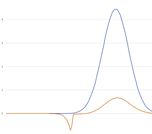
There are segments of the graph where the area under the blue line is very small but the area under the orange line is large, and that's our black swan; what we want is a distribution that samples from regions where the orange area is large, and if possible skips regions where it is small. That is, we consider the large-area regions important contributors to the expected value, and the small-area regions unimportant contributors; we wish to target our samples so that no important regions are ignored. That's why this technique for computing expected value is called "importance sampling".

Exercise: The uniform distribution is pretty good on the key requirement that it never be small when the area under the orange line is large, because it is always the same size from 0.0 to 1.0; that's why it is the uniform distribution, after all. It's not great on our second measure; it spends around 30% of its time sampling from regions where the orange line has essentially no area under it.

Write some code that tries different distributions. For example, implement the distribution that has weight function x => (0 <= x && x <= 1) ? x : 0

(Remember that this is not a normalized distribution, so you'll have to compute nq.)

Does that give us an even better estimate of the expected value of f?

Something to ponder while you're working on that: what would be the ideal choice of distribution?

Summing up:

• Suppose we have a weighted distribution of doubles p and a function from double to double f.
• We wish to accurately estimate the average value of f when it is applied to a large set of samples from p; this is the expected value.
• However, there may be "black swan" regions where the value of f is important to the average, but the probability of sampling from that region is low, so our average could require a huge number of samples to get an accurate average.
• We can fix the problem by choosing any weighted distribution q that has the same support as pbut is more likely to sample from important regions.
• The expected value of g (given above) over samples drawn from q is the same as the expected value of fover samples from p.

This is great, and I don't know if you noticed, but I removed any restriction there that p or q be distributions only on 0.0 to 1.0; this technique works for weighted distributions of doubles over any support!

Aside: We can weaken our restriction that q have the same support as p; if we decide that q can have zero weight for particularly unimportant regions, where, say, we know that f(x)*p.Weight(x) is very small, then that's still going to produce a good estimate.

Aside: Something I probably should have mentioned before is that all of the techniques I'm describing in this series for estimating expected values require that the expected value exists! Not all functions applied to probability distributions have an expected value because the average value of the function computed on a group of samples might not converge as the size of the group gets larger. An easy example is, suppose we have a standard normal distribution as our p" and x => 1.0 / p.Weight(x) as our f. The more samples from p we take, the more likely it is that the average value of f gets larger!

However, it's not all sunshine and roses. We still have two problems, and they're pretty big ones:

• How do we find a good-quality q distribution?
• We need to know the normalization constants for both distributions. If we do not know them ahead of time (because, say, we have special knowledge that the continuous uniform distribution is normalized) then how are we going to compute them? Area(p.Weight) or Area(q.Weight) might be expensive or difficult to compute.It seems like in the general case we still have to solve the calculus problem.

Aside: The boldface sentence in my last bullet point contains a small but important error. What is it? Leave your guesses in the comments; the answer will be in an upcoming episode.

I'm not going to implement a general-purpose importance sampling algorithm until we've made at least some headway on these remaining problems.

Next time on FAIC: It's Groundhog Day! I'm going to do this entire episode over again; we're going to make a similar argument - things equal to the same are equal to each other - but starting from a different place. We'll end up with the same result, and deduce that importance sampling works.