Life, part 10
Last time on FAIC I discussed a technique for parallelizing computation of Life grids by using SIMD instructions to handle 256 bits worth of grid state truly in parallel. Today I'm going to not present an implementation, but rather discuss how the Life problem is one that is ideally suited for existing hardware acceleration that many PC users have on their machines already.
I've often marveled at the technology that goes into monitors and the computers that they're plugged into. I have two 1920*1080 monitors hooked up to my machine right now. They refresh the screens 60 times a second, and there is typically 4 to 6 bytes of colour information sent per pixel; let's be conservative and say 4. So that is:
2 x 1920 x 1080 x 60 x 4 = just under one billion bytes per second
and that's for my simple little two-monitor setup! I could have more monitors at higher resolution and higher refresh rates easily enough.
How on earth do computers keep up, particularly for something like a game where there are many computations to make to determine the value of each pixel on each screen refresh?
The answer of course is that we've built specialized hardware that attacks the problem of apply a function to every one of this grid of pixels in parallel". Today I want to describe one of the most basic operations that can be handled by highly optimized parallel hardware by restricting the function at hand to a very particular set of functions called convolutions.
Aside: I note that we'll be discussing discrete convolutions today; there is also a whole theory of continuous convolutions in signal processing theory that does not concern us.
The terminology is somewhat intimidating, but convolutions are actually very simple when you see how they work. For our purposes today a convolution is a function that takes two arguments, both two-dimensional arrays.
The first argument is called the kernel. It is typically small, typically square, and typically has an odd side length; 3*3 is common and without loss of generality, we'll look just at 3*3 kernels today. Its values are numbers; for our purposes let's suppose they are floating point numbers.
The second argument is an two-dimensional array with one value per pixel being computed. Think of it as the input screen". For our purposes, let's suppose they are integers.
The output of the function is a new array of values, one per pixel. Think of it as the output screen", and it is also a two-dimensional array of integers.
What then is the function that takes these two arguments? The idea is very straightforward.
- For each pixel in the input, imagine overlaying" the kernel on that pixel so that the center of the kernel array is over the pixel.
- Multiply each value in the kernel with the corresponding input pixel below" it.
- Take the sum of the products.
- That's the value for the corresponding output pixel.
Let's work an example.
Suppose our input is a two-dimensional array corresponding to this greyscale 32 x 32 bitmap which I have blown up to examine the detail:
All of these input values are 255 (the white) or 0 (the black).
Let's suppose our kernel is
0.0625 0.125 0.06250.125 0.25 0.1250.0625 0.125 0.0625
That is, 1/16th, 1/8th, 1/16th, and so on.
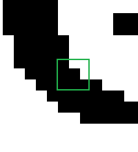
Now we can compute the convolution. Remember, we're going to do the same operation on every pixel: overlay the kernel centered on the pixel, multiply corresponding values, sum them up. Let's suppose the current pixel we are looking at is the one in the center of the nine pixels I've highlighted below:
The situation is as follows:
kernel overlaid on product (rounded)0.0625 0.125 0.0625 0 255 255 0 32 16 0.0625 0.25 0.0625 0 0 255 0 0 160.0625 0.125 0.0625 0 0 0 0 0 0
The sum of the products is 64, so the old value of this pixel is the 0 in the center and the new value is 64.
Now suppose we applied that process to every pixel in the bitmap and then displayed the output bitmap as a grayscale:
We blurred it! This particular blur is called 3*3 Gaussian" and it is extremely common in graphics processing. There are many other common kernels for blurring, sharpening, edge detection, brightening, dimming, and so on. Basically the idea here is that the new value of every pixel is a weighted average of the nearby pixels; precisely how you choose those weights determines what image operation the particular convolution with that kernel performs.
That is maybe all very interesting and the next time you play some video game you can notice all the places in which graphical elements are blurred or sharpened or dimmed or whatever. But why is this relevant to Life?
Because if you take as your kernel
1 1 11 9 11 1 1
then the convolution of a Life grid with that kernel is a new grid of numbers that should seem familiar; as I mentioned at the end of episode 7, all the places in the output array that have the value 3, 10 or 11 are living cells in the next tick, and everything else is dead. The 3s are dead cells with three living neighbours, the 10s and 11s are living cells with two and three neighbours.
(Thanks once again to reader yurivkhan, whose comment on part six inspired me to add this episode; I was not initially planning on discussing image processing, but I am glad I did.)
Now, there are some issues to worry about. I completely glossed over what happened on the edges of that blur, for example. The definition of the convolution function I gave assumed that the overlaying of the kernel on the image actually overlapped, and in real graphics processing you need to specify what happens when the kernel goes over an edge".
What I did of course was I skipped running the convolution entirely on the edges and just kept them white. For our Life implementation, were we to use this technique, we'd probably do something similar to keep the edge permanently dead.
UPDATE: Reader Shawn Hargreaves pointed me at a sample application showing how to implement Life in C# using a convolution on a GPU, which you can find here. The kernel they are using is
2 2 22 1 22 2 2
Which, similarly, produces 5 if the cell is alive with two neighbours, 6 if dead with three neighbours, and 7 if alive with three neighbours; those cells are living in the next generation and the rest are dead. Notice also that the convolution definition specifies what edge processing algorithm to use along with the kernel. Thanks Shawn!
If we had special-purpose software libraries and hardware that could compute convolutions on large grids extremely quickly, then we could use that to get a big marginal speedup in our Life algorithms.
How big is big"?
I am not set up to do GPU experiments on my little gaming machine here, but even cheap gaming machine GPUs can run a convolution at a rate of many hundred millions of pixels per second. Back in 2013 a graduate student did a fascinating writeup on optimizing Life on a GPU and managed to get an astonishing 20 billion cell computations per second. However, that throughput was only attained when the grid sizes became quite large, and there was considerable optimization work done to attain a fast kernel function that worked on grids that stored cells as bits.
Let's do a quick back-of-the-envelope to see how that compares to our efforts so far.
- My best implementation so far did 5000 generations of 64k cells in 3.25 seconds, so that's 100 million cells per second. The optimized GPU reported in 2013 is 200x faster.
- Jeroen's SIMD did 5 million generations of 256 cells in 1 second, so that's about 1.3 billion cells per second - though there is a bit caveat here that the program can only do 16*16 grids! A program that used SIMD instructions on larger grids would be a bit slower than 1.3 billion cells per second, but it would be in that neighbourhood. The optimized GPU is on the order of 20x faster.
I keep on coming back to this main theme: adding raw power to improve the marginal performance of an algorithm can only go so far, and we're seeing here what the limits of that are. We are not going to do better than GPUs on any variation of the Life algorithm that works by examining every cell in a finite grid in order to determine the next tick's grid state. GPUs are the best available technology for parallelizing simple math operations onto grids where the new cell value is a function of the near neighbours of each cell.
Moreover, an increase in speed by 200x again just means that if our previous implementation is in its performance budget for an n-quad, then throwing a GPU at the problem means that we can now do an n+3 or n+4-quad in the same time budget.
And also it is worth remembering that a GPU only has so much addressable memory on board! One expects that a typical GPU might handle something like an 8192*8192 image - a 13-quad - before it runs out of space.
We've found a rough upper bound on how good we can make any variation on the naive examine every cell every time" algorithm. If we want to get better speed, we're going to have to stop looking at every cell and counting its neighbors.
Next time on FAIC: All that said, I'm going to look at one more algorithm that examines every cell every time, but we will at least make a start at using specific characteristics of the Life problem in order to do less work. We will take an insight from this episode and see if we can use it to advantage to get a marginal advantage, and then use that as the basis for further improvements in coming episodes. Stay tuned!


