Life, part 22

Code for this episode is here.

So far in this series every algorithm we've attempted has been either O(cells) or O(changes) in time, and O(cells) in space. Going with a straightforward big square with dead cells surrounding it" approach tends to use up a lot of space as the side of the square grows larger.

Is there a way to make the space usage asymptotically smaller, say, O(living cells)? Then we could have arbitrarily large boards and know that we are only paying for the cells that are alive. Of course it would certainly be nice if the step time was still O(changes) while we're at it.

Before I get into that though, a quick note about the UI; I've added the ability for the different Life engines to report statistics to the UI such as generation count, number of changed cells on the previous generation, or anything else that might be of interest while watching a pattern evolve. If you're playing around with the engines, consider using this rather simple new feature to try to gain some insight into their behaviours.

The code is straightforward; if a Life engine implements an interface IReport then IReport.Report is called every time the UI updates; easy peasy.

After writing today's implementation I came across this charmingly straightforward similar Life implementation in Python, on Madelyn Eriksen's blog. As Madelyn points out, rather than going with a dense" array that is over 50% dead cells almost always, we could instead use a sparse" array; that is, simply make a collection of the coordinates of the living cells, and spend no space at all representing the empty ones.

That's O(living cells) in memory size, obviously. But what about the time cost? The Python implementation given is also O(living cells) per tick, not O(changes). The implementation of a sparse array algorithm that is O(living cells) in space and O(changes) in time is straightforward so let's just go for it!

Our basic data structures are: a set of living cells, a set of recently born cells, and a set of recently died cells:

class SparseArray : ILife, IReport{ private HashSet<(long, long)> living; private HashSet<(long, long)> recentBirths; private HashSet<(long, long)> recentDeaths; private int generation; public SparseArray() { Clear(); } public void Clear() { living = new HashSet<(long, long)>(); recentBirths = new HashSet<(long, long)>(); recentDeaths = new HashSet<(long, long)>(); generation = 0; }

Nothing at all surprising about that.

Our getter and setter indexers can, for the first time in this series, skip checking whether the coordinates are valid:

 public bool this[long x, long y] { get => living.Contains((x, y)); set { if (value) { if (living.Add((x, y))) recentBirths.Add((x, y)); } else { if (living.Remove((x, y))) recentDeaths.Add((x, y)); } } }

And now our step algorithm is just as you'd expect: for each previously-changed cell, check to see if it or any of its neighbours need to change on this tick. If so, record them into brand-new recent births" and recent deaths" sets that will be the change list for the next generation.

Updating the living set with the changes is two built-in set operations.

 public void Step() { var previousBirths = recentBirths; recentBirths = new HashSet<(long, long)>(); var previousDeaths = recentDeaths; recentDeaths = new HashSet<(long, long)>(); foreach ((long x, long y) in previousBirths) CheckCellAndNeighbours(x, y); foreach ((long x, long y) in previousDeaths) CheckCellAndNeighbours(x, y); living.UnionWith(recentBirths); living.ExceptWith(recentDeaths); generation += 1; }

And of course our check the cell and its neighbours" function is very similar to code we've seen several times already in this series:

 private void CheckCellAndNeighbours(long x, long y) { for (int iy = -1; iy < 2; iy += 1) { long cy = y + iy; for (int ix = -1; ix < 2; ix += 1) { long cx = x + ix; bool state = this[cx, cy]; int nw = this[cx - 1, cy - 1] ? 1 : 0; int n = this[cx, cy - 1] ? 1 : 0; int ne = this[cx + 1, cy - 1] ? 1 : 0; int w = this[cx - 1, cy] ? 1 : 0; int e = this[cx + 1, cy] ? 1 : 0; int sw = this[cx - 1, cy + 1] ? 1 : 0; int s = this[cx, cy + 1] ? 1 : 0; int se = this[cx + 1, cy + 1] ? 1 : 0; int count = nw + n + ne + w + e + sw + s + se; if (state & count != 2 & count != 3) recentDeaths.Add((cx, cy)); else if (!state & count == 3) recentBirths.Add((cx, cy)); } } }}

An interesting point about this implementation: I said near the start of this series that I was not going to implement wrap around" semantics, but I suppose I have here; since I have no bounds checks on the coordinates at all, we'll wrap around" if we go over the maximum value of a long. I'm not too worried about it.

That was a very short and sweet implementation compared to the bit-twiddly, repetitive, table-driven code we had to write for Stafford's algorithm! But I want to consider the memory and time performance of this algorithm.

The memory performance is asymptotically pretty good; plainly the memory used is proportional to the number of living cells, which we have not seen before in this series. However we should also consider that proportion. For Abrash's algorithm we had one byte per cell, living or dead (though we only used six of the eight bits). For Stafford's algorithm we similarly used 15 bits of a 16 bit short to store three cells, so that's five bits per cell. As I mentioned last time, David Stafford emailed me and described some schemes whereby one could compress that even further to store more neighbour counts and cell state in fewer bits.

This scheme uses a massive 128 bits - two longs - per living cell! Now, it uses nothing at all for the dead cells, which is great, but still, 128 is a lot. And that's not counting all the overhead of maintaining the internal data structures of the hash set, which are also O(living cells) additional burden of unknown size. (I mean, I could work it out by reading the hash set source code, but I'm not going to.)

The up side of course is we get the full two-to-the-128 cells available in our 64-quad, but it seems like we are using a bunch of memory here. There are things we could do about that. We could have a (short, short) dictionary for all the cells inside a 16-quad, for example, which seems pretty reasonable, and now we're down to 32 bits per living cell instead of 128; we could then have a sparse array of 16-quads, and so on; you see how it goes I'm sure. This could get quite complex, but we could get it down to a relatively smaller number of bits per living cell if we tried.

What's your intuition about the wall-clock performance of this algorithm on our standard performance problem of 5000 generations of acorn"? Give that some thought and then scroll down for the results to see if you were right.

.

.

.

.

.

.

Algorithm time(ms) ticks size(quad) megacells/sNaive (Optimized): 4000 5K 8 82Abrash 550 5K 8 596Abrash w/ changes 190 5K 8 1725 Abrash, O(c) 240 5K 8 1365Stafford 180 5K 8 1820SparseArray 4000 5K 64 ?

We are back to the time performance of our original (slightly optimized) naive array implementation! Once again we are doing a dozen set operations per step per change, just as we were doing dozens of array operations per cell in the naive implementation. Those set operations are more expensive than array operations, so the fact that we are doing fewer operations by only looking at changed cells is balanced out by the increased cost per operation.

It's now not clear what megacells per second" means now that the board size is essentially unlimited.

We could do this entire series over again; instead of starting with regular rectangular arrays as our basic data structure, we could start with sets and dictionaries. We could have a dictionary mapping (long, long) to (count, bool) and update neighbour counts on changes as we did in Abrash's algorithm; we could make a sparse array version of Stafford's algorithm. We would make the memory burden of those algorithms proportional to the number of living cells, but in every case I am quite sure we would see a significant time performance penalty for going with hash sets over normal arrays.

Though it would be interesting to try and then compare the sparse vs dense array implementations, this series is already far longer than I thought it would be, and we still have at least two more implementations to get through; let's move forward rather than revisiting ground we've already covered.

Next time on FAIC: We'll look at a new idea for a lookup-table based Life algorithm.

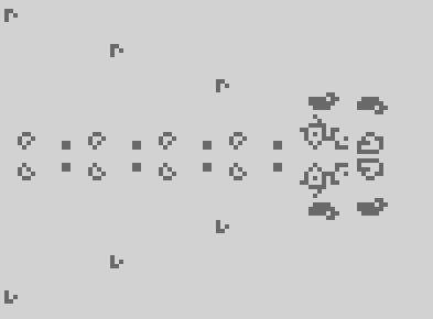
For today's extra content: a few episodes back we were talking about puffers, and I mentioned that the first puffer found leaves behind some blinkers and bookends:

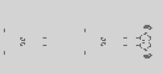
Fun fact: if you add another couple of spaceships to run alongside puffer1, the debris becomes loafs, blocks and gliders!

This is a simplified version of the pattern backrake 3". It has a number of interesting uses, which we will get to in upcoming episodes.