Circles to Circles

This post expands on something I said in passing yesterday. I said in the body of the post that

... the image of a circle in the complex plane under a Mobius transformation is another circle.

and added in a footnote that

For this to always be true, you have to include a line as a special case of a circle, a circle of infinite radius if you like.

This post will illustrate these statements with Python code and plots. First, some code for drawing circles and other curves in the complex plane.

 from numpy import exp, pi, linspace import matplotlib.pyplot as plt  = linspace(0, 2*pi, 200) def circle(radius, center): return center + radius*exp(1j*) def plot_curves(curves): for c in curves: plt.plot(c.real, c.imag) plt.axes().set_aspect(1) plt.show() plt.close()

Next, code for Mobius transformations, and the particular Mobius transformation we'll use in our plots.

 def mobius(z, a, b, c, d): return (a*z + b)/(c*z + d) def m(curve): return mobius(curve, 1, 2, 3, 4)

Now we'll plot three circles and their images under the Mobius transformation

m(z) = (z + 2)/(3z + 4)

with the following code.

 circles = [circle(1, 0), circle(2, 0), circle(2, 2)] plot_curves(circles) plot_curves([m(c) for c in circles])

This produces

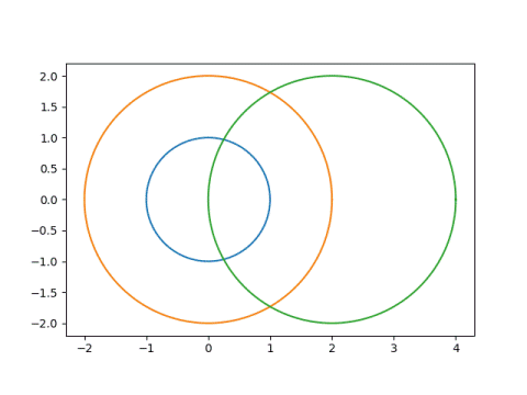
and

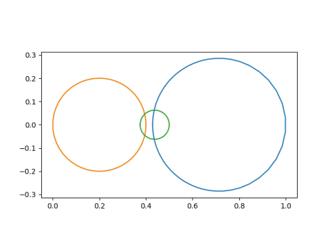
Notice that the first circle, in blue, started out as the smallest circle and was contained inside the second circle, in orange. But in the image, the blue circle became the largest, and is no longer inside the orange circle. That is because our Mobius transformation has a singularity at -4/3, and things get turned inside-out around that point.

Next we'll look at an example of lines being mapped to lines.

 line = linspace(-100, 100, 600) curves = [line, 1j*line - 4/3] plot_curves(curves) plot_curves([m(c) for c in curves])

This produces

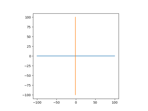
and

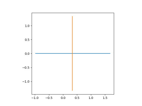
These lines are mapped to lines because they both pass through the singularity at -4/3. The real axis, in blue, is mapped to itself. The line -4/3 + iy, is shifted over to have real part 1/3.

Finally, lets look at lines being mapped to circles. Since the inverse of a Mobius transformation is another Mobius transformation, this example also shows that circles can be mapped to lines.

 lines = [1j*line - 4, 1j*line + 4, line - 4j, line + 4j] plot_curves(lines) plot_curves([m(c) for c in lines])

This produces

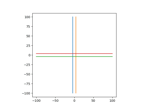
and

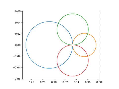
Note that the circles don't quite close. That's because my line only runs from -100 to 100, not - to . The gap in the circles is at 1/3, because that's the limit of our transformation (z + 2)/(3z + 4) as z goes to .

To illustrate things further, I'd like to look at a smiley face and what happens to it under different Mobius transformations.

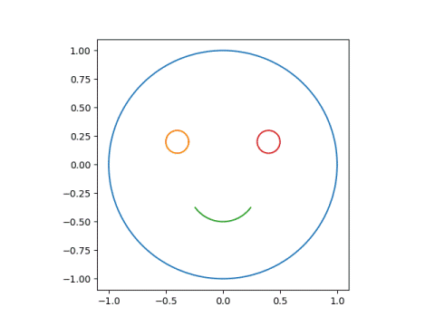
Here's the code to draw the original face.

 dash = linspace(0.60, 0.90, 20) smile = 0.3*exp(1j*2*pi*dash) - 0.2j left_eye = circle(0.1, -0.4+.2j) right_eye = circle(0.1, 0.4+.2j) face = [circle(1, 0), left_eye, smile, right_eye]

Next, let's subject this face to the Mobius transformation with parameters (1, 0, 1, 3). The singularity is at -3, outside the face and fairly far away.

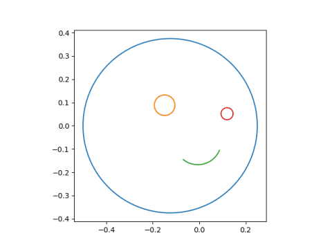
Next we'll use parameters (1, 0, 1, -1+1j), which has a sigularity at 1 - i, closer to the face, and hence more distortion.

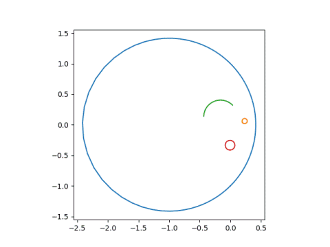
Now we use parameters (1, 0, 3, 1), putting the singularity at -1/3, inside the face.

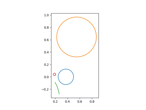
Finally, we look at parameters (1, 0, 1, 0.4-0.2j), putting the singularity inside the left eye.

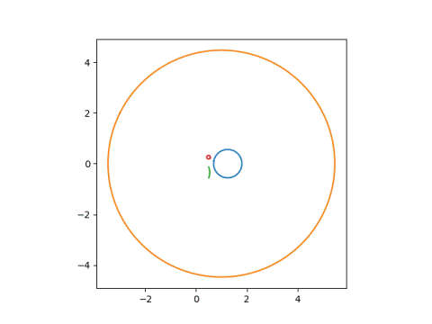
The next post explains how to pick the parameters of a Mobius transformation to make points go where you want.

The post Circles to Circles first appeared on John D. Cook.