Reproducing a geometry theorem diagram

I ran across a geometry theorem with the following diagram.

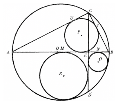
The theorem corresponding to the diagram is interesting, but I found reproducing the diagram more interesting.

The segmentAB is a diameter and the lineCD is perpendicular to the diameter.

Assume the outer circle is a unit circle. I guessedC = (cos(1), sin(1)) and made the following diagram.

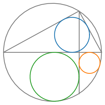
I guessed the value of C by eyeballing it, but in retrospect this would have been a convenient value for the creator of the original diagram to have chosen.

Drawing the blue circle inscribed in the triangle was easy using the equations for the center and radius from this post. Drawing the other two circles, the green and orange circles, was harder. They are also inscribed circles, but not inscribed in a triangle. They're inscribed in a three-sided figure with two perpendicular sides and a circular arc.

The radius r of the green circle is the distance from the center of the circle to each of its tangent lines. Also, the distance from the origin to the center of the circle must be 1 - r. This is enough information to set up a quadratic equation forr. The same reasoning applies to the orange circle.

The original diagram comes from [1] and the theorem it illustrates says the diameter of the blue circle equals the sum of the radii of the green and orange circles.

Python code

In case you're interested, here's the code that created the diagram.

#!/usr/bin/env -S uv run --script# /// script# dependencies = ["numpy", "matplotlib"]# ///import numpy as npimport matplotlib.pyplot as pltdef connect(A, B, color='gray'): plt.plot([A[0], B[0]], [A[1], B[1]], color=color, linewidth=2)def circle(c, r, color='gray'): t = np.linspace(0, 2*np.pi) plt.plot(c[0] + r*np.cos(t), c[1] + r*np.sin(t), color=color, linewidth=2)def quadratic(a, b, c): det = b**2 - 4*a*c return ((-b - det**0.5)/(2*a), (-b + det**0.5)/(2*a))A = np.array([-1, 0])B = np.array([ 1, 0])C = np.array([np.cos(1), np.sin(1)])a = np.linalg.norm(B - C)b = np.linalg.norm(A - C)c = np.linalg.norm(B - A)s = (a + b + c)/2circle([0,0], 1)connect(A, B,)connect(A, C)connect(C, B)connect(C, C*np.array([1, -1]))center = (a*A + b*B + c*C)/(2*s)radius = 0.5*a*b/scircle(center, radius, 'C0')Ex = C[0]roots = quadratic(1, 2 + 2*Ex, Ex**2 - 1)r = roots[1] # Smaller root is negaiveprint(roots)center = (r + Ex, -r)circle(center, r, 'C1')roots = quadratic(1, 2 - 2*Ex, Ex**2 - 1)r = roots[1] # Smaller root is negaivecenter = (Ex - r, -r)circle(center, r, 'C2')plt.gca().set_aspect("equal")plt.axis("off")plt.show()

[1] Leon Bankoff. A Geometrical Coincidence. Mathematics Magazine, Vol. 37, No. 5 (Nov., 1964), p. 324.

The post Reproducing a geometry theorem diagram first appeared on John D. Cook.