How to digitize a graph

Suppose you have a graph of a function, but you don't have an equation for it or the data that produced it. How can you reconstruction the function?

There are a lot of software packages to digitize images. For example, Web Plot Digitizer is one you can use online. Once you have digitized the graph at a few points, you can fit a spline to the points to approximately reconstruct the function. Then as a sanity check, plot your reconstruction to see if it looks like the original. It helps to have the same aspect ratio so you're not distracted by something that doesn't matter, and so that differences that do matter are easier to see.

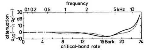
For example, here is a graph from Zwicker and Fastl's book on psychoacoustics. It contains many graphs with no data or formulas. This particular one gives the logarithmic transmission factor between free field and the peripheral hearing system.

Here's Python code to reconstruct the functions behind these two curves.

import matplotlib.pyplot as pltimport numpy as npfrom scipy import interpolate curve_names = ["Free", "Diffuse"]plot_styles = { "Free" : 'b-', "Diffuse" : 'g:'}data = {}for name in curve_names: data = np.loadtxt("{}.csv".format(name), delimiter=',') x = data[:,0] y = data[:,1] spline = interpolate.splrep(x, y) xnew = np.linspace(0, max(x), 100) ynew = interpolate.splev(xnew, spline, der=0) plt.plot(xnew, ynew, plot_styles[name]) logical_x_range = 24 # Barklogical_y_range = 40 # dBphysical_x_range = 7 # inchphysical_y_range = 1.625 # inchplt.legend(curve_names, loc=2)plt.xlabel("critical-band rate")plt.ylabel("attenuation")plt.xlim((0, logical_x_range))plt.axes().set_aspect( (physical_y_range/logical_y_range) / (physical_x_range/logical_x_range) )ax = plt.gca()ax.get_xaxis().set_ticks([0, 4, 8, 12, 16, 20, 24])ax.get_yaxis().set_ticks([-10, 0, 10, 20, 30])plt.show()

Here's the reconstructed graph.