Nearly all the area in a high-dimensional sphere is near the equator

Nearly all the area of a high-dimensional sphere is near the equator. And by symmetry, it doesn't matter which equator you take. Draw any great circle and nearly all of the area will be near that circle. This is the canonical example of "concentration of measure."

What exactly do we mean by "nearly all the area" and "near the equator"? You get to decide. Pick your standard of "nearly all the area," say 99%, and your definition of "near the equator," say within 5 degrees. Then it's always possible to take the dimension high enough that your standards are met. The more demanding your standard, the higher the dimension will need to be, but it's always possible to pick the dimension high enough.

This result is hard to imagine. Maybe a simulation will help make it more believable.

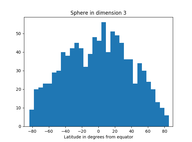
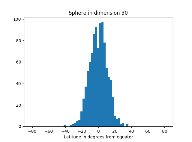
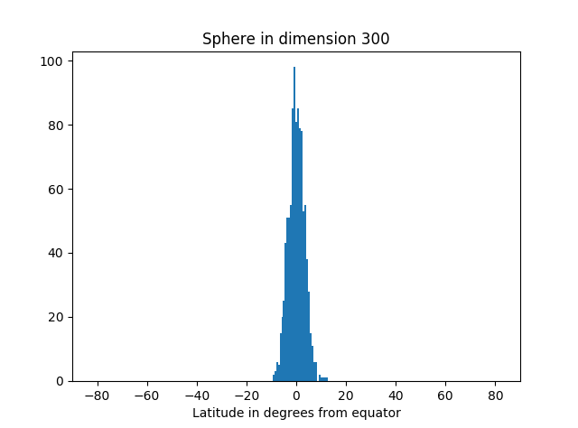
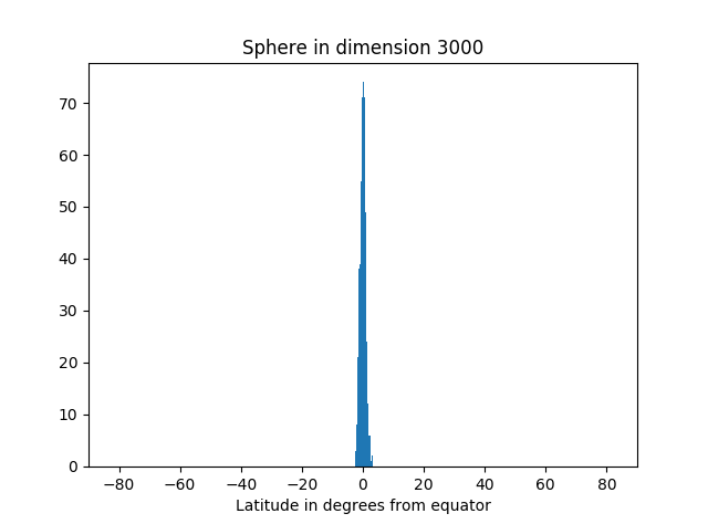
In the simulation below, we take as our "north pole" the point (1, 0, 0, 0, ", 0). We could pick any unit vector, but this choice is convenient. Our equator is the set of points orthogonal to the pole, i.e. that have first coordinate equal to zero. We draw points randomly from the sphere, compute their latitude (i.e. angle from the equator), and make a histogram of the results.

The area of our planet isn't particularly concentrated near the equator.

But as we increase the dimension, we see more and more of the simulation points are near the equator.

Here's the code that produced the graphs.

from scipy.stats import normfrom math import sqrt, pi, acos, degreesimport matplotlib.pyplot as pltdef pt_on_sphere(n): # Return random point on unit sphere in R^n. # Generate n standard normals and normalize length. x = norm.rvs(0, 1, n) length = sqrt(sum(x**2)) return x/lengthdef latitude(x): # Latitude relative to plane with first coordinate zero. angle_to_pole = acos(x[0]) # in radians latitude_from_equator = 0.5*pi - angle_to_pole return degrees( latitude_from_equator )N = 1000 # number of samplesfor n in [3, 30, 300, 3000]: # dimension of R^n latitudes = [latitude(pt_on_sphere(n)) for _ in range(N)] plt.hist(latitudes, bins=int(sqrt(N))) plt.xlabel("Latitude in degrees from equator") plt.title("Sphere in dimension {}".format(n)) plt.xlim((-90, 90)) plt.show()

Not only is most of the area near the equator, the amount of area outside a band around the equator decreases very rapidly as you move away from the band. You can see that from the histograms above. They look like a normal (Gaussian) distribution, and in fact we can make that more precise.

If A is a band around the equator containing at least half the area, then the proportion of the area a distance r or greater from A is bound by exp( -(n-1)r^2 ). And in fact, this holds for any set A containing at least half the area; it doesn't have to be a band around the equator, just any set of large measure.

Related post: Willie Sutton and the multivariate normal distribution