Fixing Random, part 33

Last time on FAIC I showed why our naive implementation of computing the expected value can be fatally flawed: there could be a "black swan" region where the "profit" function f is different enough to make a big difference in the average, but the region is just small enough to be missed sometimes when we're sampling from our distribution p

The obvious solution is to work harder, not smarter: just do more random samples when we're taking the average! But doesn't it seem to be a little wasteful to be running ten thousand samples in order to get 9990 results that are mostly redundant and 10 results that are extremely relevant outliers?

Perhaps we can be smarter.

We know how to compute the expected value in a discrete non-uniform distribution of doubles: multiply each value by its weight, sum those, and divide by the total weight. But we should think for a moment about why that works.

If we have an unfair two-sided die - a coin - stamped with value 1.23 on one side, and -5.87 on the other, and 1.23 is twice as likely as -5.87, then that is the same as a fair three sided die - whatever that looks like - with 1.23 on two sides and -5.87 on the other. One third of the time we get the first 1.23, one third of the time we get the second 1.23, and one third of the time we get -5.87, so the expected value is 1.23/3 + 1.23/3 - 5.87/3, and that's equivalent to (2 * 1.23 - 5.87) / 3. This justifies our algorithm.

Can we use this insight to get a better estimate of the expected value in the continuous case? What if we thought about our continuous distribution as just a special kind of discrete distribution?

Aside: In the presentation of discrete distributions I made in this series, of course we had integer weights. But that doesn't make any difference in the computation of expected value; we can still multiply values by weights, take the sum, and divide by the total weight.

Our original PDF - that shifted, truncated bell curve - has support from 0.0 to 1.0. Let's suppose that instead we have an unfair 1000-sided die, by dividing up the range into 1000 slices of size 0.001 each.

• The weight of each side of our unfair die is the probability of rolling that side.
  • Since we have a normalized PDF, the probability is the area of that slice.
  • Since the slices are very thin, we can ignore the fact that the top of the shape is not "level"; let's just treat it as a rectangle.
  • The width is 0.001; the height is the value of the PDF at that point.
  • That gives us enough information to compute the area.
• Since we have a normalized PDF, the total weight that we have to divide through is 1.0, so we can ignore it. Dividing by 1.0 is an identity.
• The value on each side of the die is the value of our profit function at that point.

Now we have enough information to make an estimate of the expected value using our technique for discrete distributions.

Aside: Had I made our discrete distributions take double weights instead of integer weights, at this point I could simply implement a "discretize this distribution into 1000 buckets" operation that turns weighted continuous distributions into weighted discrete distributions.

However, I don't really regret making the simplifying choice to go with integer weights early in this series; we're immediately going to refactor this code away anyways, so turning it into a discrete distribution would have been a distraction.

Let's write the code: (Code for this episode is here.)

public static double ExpectedValue(
this IWeightedDistribution<double> p,
Func<double, double> f) =>
// Let's make a 1000 sided die:
Enumerable.Range(0, 1000)
// " from 0.0 to 1.0:
.Select(i => ((double)i) / 1000)
// The value on the "face of the die" is f(x)
// The weight of that face is the probability
// of choosing this slot
.Select(x => f(x) * p.Weight(x) / 1000)
.Sum();
// No need to divide by the total weight since it is 1.0.

And if we run that:

Console.WriteLine($"{p.ExpectedValue(f):0.###}");

we get

0.113

which is a close approximation of the true expected value of this profit function over this distribution. Total success, finally!

Or, maybe not.

I mean, that answer is correct, so that's good, but we haven't solved the problem in general.

The obvious problem with this implementation is: it only works on normalized distributions whose support is between 0.0 and 1.0. Also, it assumes that 1000 is a magic number that always works. It would be nice if this worked on non-normalized distributions over any range with any number of buckets.

Fortunately, we can solve these problems by making our implementation only slightly more complicated:

public static double ExpectedValue(
this IWeightedDistribution<double> p,
Func<double, double> f,
double start = 0.0,
double end = 1.0,
int buckets = 1000)
{
double sum = 0.0;
double total = 0.0;
for (int i = 0; i < buckets; i += 1)
{
double x = start + (end - start) * i / buckets;
double w = p.Weight(x) / buckets;
sum += f(x) * w;
total += w;
}
return sum / total;
}

That totally works, but take a closer look at what this is really doing. We're computing two sums, sum and total, in exactly the same manner. Let's make this a bit more elegant by extracting out the summation into its own method:

public static double Area(
Func<double, double> f,
double start = 0.0,
double end = 1.0,
int buckets = 1000) =>
Enumerable.Range(0, buckets)
.Select(i => start + (end - start) * i / buckets)
.Select(x => f(x) / buckets)
.Sum();
public static double ExpectedValue(
this IWeightedDistribution<double> p,
Func<double, double> f,
double start = 0.0,
double end = 1.0,
int buckets = 1000) =>
Area(x => f(x) * p.Weight(x), start, end, buckets) /
Area(p.Weight, start, end, buckets);

As often happens, by making code more elegant, we gain insights into the meaning of the code. That first function should look awfully familiar, and I've renamed it for a reason. The first helper function computes an approximation of the area under a curve; the second one computes the expected value as the quotient of two areas.

It might be easier to understand it with a graph; here I've graphed the distribution p.Weight(x) as the blue line and the profit times the distribution f(x) * p.Weight(x)as the orange line:

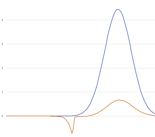
The total area under the blue curve is 1.0; this is a normalized distribution.

The orange curve is the blue curve multiplied by the profit function at that point. The total area under the orange curve - remembering that area below the zero line is negative area - divided by the area of the blue curve (1.0) is the expected value.

Aside: You can see from the graph how carefully I had to contrive this "black swan" scenario. I needed a region of the graph where the area under the blue line is close to 0.001 and the profit function is so negative that it makes a large negative area there when multiplied, but without making a large negative area anywhere else.

Of course this example is contrived, but it is not unrealistic; unlikely things happen all the time, and sometimes those unlikely things have important consequences.

An interesting feature of this scenario is: look at how wide the negative region is! It looks like it is around 10% of the total support of the distribution; the problem is that we sample from this range only 0.1% of the time because the blue line is so low here. We'll return to this point in the next episode.

Aside: The day I wrote this article I learned that this concept of computing expected value of a function applied to a distribution by computing the area of the product has a delightful name: LOTUS, which stands for the Law Of The Unconscious Statistician.

The tongue-in-cheek name is apparently because statistics students frequently believe that "the expected value is the area under this curve" is the definition of expected value. I hope I avoided any possible accusation of falling prey to the LOTUS fallacy. We started with a correct definition of expected value: the average value of a function applied to a bunch of samples, as the size of the bunch gets large. I then gave an admittedly unrigorous, informal and hand-wavy justification for computing it by approximating area, but it was an argument.

We've now got two ways of computing an approximation of the expected value when given a distribution and a function:

• Compute a bunch of samples and take their average.
• Compute approximate values of two areas and divide them.

As we know, the first has problems: we might need a very large set of samples to find all the relevant "black swan" events, and therefore we spend most of our time sampling the same boring high-probability region over and over.

However, the second has some problems too:

• We need to know the support of the distribution; in my contrived example I chose a distribution over 0.0 to 1.0, but of course many distributions have much larger ranges.
• We need to make a guess about the appropriate number of buckets to get an accurate answer.
• We are doing a lot of seemingly unnecessary math; between 0.0 and, say 0.3, the contribution of both the blue and orange curves to the total area is basically zero. Seems like we could have skipped that, but then again, skipping a region with total probability of one-in-a-thousand led to a bad result before, so it's not entirely clear when it is possible to save on work.
• Our first algorithm was fundamentally about sampling, which seems appropriate, since "average of a set of samples" is the definition of expected value. This algorithm is just doing an approximation of integral calculus; something seems "off" about that.

It seems like we ought to be able to find an algorithm for computing expected value that is more accurate than our naive algorithm, but does not rely so much on calculus.

Next time on FAIC: We'll keep working on this problem!