Fixing Random, part 38
Last time on FAIC we were attacking our final problem in computing the expected value of a function f applied to a set of samples from a distribution p. We discovered that we could sometimes do a "stretch and shift" of p, and then run importance sampling on the stretched distribution; that way we are more likely to sample from "black swan" regions, and therefore the estimated expected value is more likely to be accurate.
However, determining what the parameters to Stretch.Distribution should be to get a good result is not obvious; it seems like we'd want to do what we did: actually look at the graphs and play around with parameters until we get something that looks right.
It seems like there ought to be a way to automate this process to get an accurate estimate of the expected value. Let's take a step back and review what exactly it is we need from the helper distribution. Start with the things it must have:
- Obviously it must be a weighted distribution of doubles that we can sample from!
- That means that it must have a weight function that is always non-negative.
- And the area under its weight function must be finite, though not necessarily 1.0.
And then the things we want:
- The support of the helper distribution does not have to be exactly support of the p, but it's nice if it is.
- The helper's weight function should be large in ranges where f(x) * p.Weight(x) bounds a large area, positive or negative.
- And conversely, it's helpful if the weight function is small in areas where the area is small.
Well, where is the area likely to be large? Precisely in the places where Abs(f(x)*p.Weight(x)) is large. Where is it likely to be small? Where that quantity is small" so"
why don't we use that as the weight function for the helper distribution?
Great Scott, why didn't we think of that before?
Aside: As I noted before in this series, all of these techniques require that the expected value actually exist. I'm sure you can imagine functions where f*p bounds a finite area, so the expected value exists, but abs(f*p) does not bound a finite area, and therefore is not the weight function of a distribution. This technique will probably not work well in those weird cases.
If only we had a way to turn an arbitrary function into a non-normalized distribution we could sample from" oh wait, we do. (Code is here.)
var p = Normal.Distribution(0.75, 0.09);
double f(double x) => Atan(1000 * (x - .45)) * 20 - 31.2;
var m = Metropolis<double>.Distribution(
x => Abs(f(x) * p.Weight(x)),
p,
x => Normal.Distribution(x, 0.15));
Let's take a look at it:
Console.WriteLine(m.Histogram(0.3, 1));
*** **** ***** ******* * ******* ** ********* ** ********* ** ********* ** *********** ** *********** ** ************* ** ************* *** ************** *** *************** *** *************** *** ***************** **** ******************* **** ******************** ***** *********************** ----------------------------------------
That sure looks like the distribution we want.
What happens if we try it as the helper distribution in importance sampling? Unfortunately, the results are not so good:
0.11, 0.14, 0.137, 0.126, 0.153, 0.094, ...
Recall that again, the correct result is 0.113. We're getting worse results with this helper distribution than we did with the original black-swan-susceptible distribution.
I'm not sure what has gone wrong here. I tried experimenting with different proposal distributions and couldn't find one that gave better results than just using the proposal distribution itself as the helper distribution.
So once again we've discovered that there's some art here; this technique looks like it should work right out of the box, but there's something that needs tweaking here. Any experts in this area who want to comment on why this didn't work, please leave comments.
And of course all we've done here is pushed the problem off a level; our problem is to find a good helper distribution for this expected value problem, but to do that with Metropolis, we need to find a good proposal distribution for the Metropolis algorithm to consume, so it is not clear that we've made much progress here. Sampling efficiently and accurately is hard!
I'll finish up this topic with a sketch of a rather complicated algorithm called VEGAS; this is an algorithm for solving the problem "how do we generate a good helper distribution for importance sampling knowing only p and f?"
Aside: The statement above is slightly misleading, but we'll say why in the next episode!
This technique, like quadrature, does require us to have a "range" over which we know that the bulk of the area of f(x)*p.Weight(x) is found. Like our disappointing attempt above, the idea is to find a distribution whose weight function is large where it needs to be, and small where it is not.
I am not an expert on this algorithm by any means, but I can give you a quick sketch of the idea. The first thing we do is divide up our range of interest into some number of equally-sized subranges. On each of those subranges we make a uniform distribution and use it to make an estimate of the area of the function on that subrange.
How do we do that? Remember that the expected value of a function evaluated on samples drawn from a distribution is equal to the area of the function divided by the area of the distribution. We can construct a uniform distribution to have area of 1.0, so the expected value is equal to the area. But we can estimate the expected value by sampling. So we can estimate areas by sampling too! Again: things equal to the same are equal to each other; if we need to find an area, we can find it by sampling to determine an expected value.
So we estimate the expected value of a uniform distribution restricted to each sub-range. Again, here's the function of interest, f(x)*p.Weight(x)
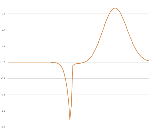
Ultimately we want to accurately find the area of this thing, but we need a black-swan-free distribution that samples a lot where the area of this thing is big.
Let's start by making some cheap estimates of the area of subranges. We'll split this thing up into ten sub-ranges, and do a super cheap estimate of the area of the subrange by sampling over a uniform distribution confined to that subrange.
Let's suppose our cheap estimate finds the area of each subrange as follows:

Now, you might say, hey, the sum of all of these is an estimate of the area, and that's what we're after; and sure, in this case it would be pretty good. But stay focussed: what we're after here with this technique is a distribution that we can sample from that is likely to have high weight where the area is high.
So what do we do? We now have an estimate of where the area of the function is big - where the expected value of the sub-range is far from zero - and where it is small.
We could just take the absolute value and stitch it all together:

And then use this as our helper distribution; as we prefer, it will be large when the area is likely to be large, and small where it is likely to be small. We'll spend almost no time sampling from 0.0 to 0.3 where the contribution to the expected value is very small, but lots of time sampling near both the big lumps.
Aside: This is an interesting distribution: it's a piecewise uniform distribution. We have not shown how to sample from such a distribution in this series, but if you've been following along, I'm sure you can see how to do it efficiently; after all, our "unfair die" distribution from way back is basically the same. You can efficiently implement distributions shaped like the above using similar techniques.
This is already pretty good; we've done ten cheap area estimates and generated a reasonably high-quality helper PDF that we can then use for importance sampling. But you've probably noticed that it is far from perfect; it seems like the subranges on the right side are either way too big or way too small, and this might skew the results.
The insight of the VEGAS algorithm's designer was: don't stop now! We have information to refine our helper PDF further.
How?
We started with ten equally-sized subranges. Numbering them from the left, it sure looks like regions 1, 2, 3, 5 and 6 were useless in terms of providing area, and regions 5 and 9 were awesome, so let's start over with ten unequally sized ranges. We'll make regions 1, 2, and 3 into one big subrange, and also regions 5 and 6 into one big subrange, and then split up regions 4, 7, 8, 9 and 10 into eight smaller regions and do it again.
Aside: The exact details of how we rebalance the subranges involve a lot of fiddly bookkeeping, and that's why I don't want to go there in this series; getting the alias algorithm right was enough work, and this would be more. Maybe in a later series I'll investigate this algorithm in more detail.
We can then keep on repeating that process until we have a helper PDF that is fine-grained where it needs to be: in the places where the area is large and changing rapidly. And it is then coarse-grained where there is not much change in area and the area is small.
Or, put another way: VEGAS looks for the spikes and the flats, and refines its estimate to be more accurate at the spikes because that's where the area is at.
And bonus, the helper PDF is always piecewise continuous uniform, which as I noted above, is relatively easy to implement and very cheap to sample from.
This technique really does generate a high-quality helper PDF for importance sampling when given a probability distribution and a function. But, it sounds insanely complicated; why would we bother?
Next time on FAIC: I'll wrap up this topic with some thoughts on why we have so many techniques for computing expected value.