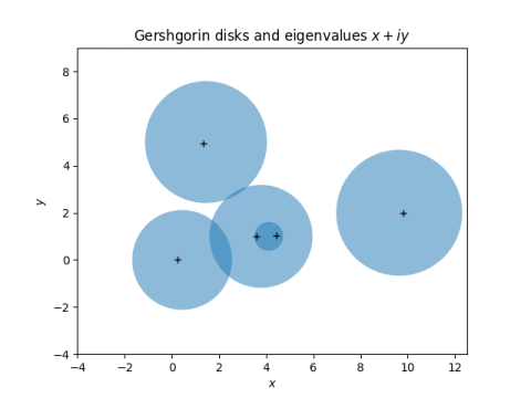
Illustrating Gershgorin disks with NumPy

Gershgorin's theorem gives bounds on the locations of eigenvalues for an arbitrary square complex matrix.

The eigenvalues are contained in disks, known as Gershgorin disks, centered on the diagonal elements of the matrix. The radius of the disk centered on the kth diagonal element is the sum of the absolute values of the elements in the kth row, excluding the diagonal element itself.

To illustrate this theorem, we create a 5 by 5 diagonal matrix and add some random noise to it. The diagonal elements are

0, 3 + i, 4 + i, 1 + 5i, 9 + 2i.

The eigenvalues of the diagonal matrix would simply be the diagonal elements. The additional random values pull the eigenvalues away from the diagonal values, but by an amount no more than Gershgorin predicts.

Note that in this example, two of the eigenvalues land in the smallest disk. It's possible that a disk may not contain any eigenvalues; what Gershgorin guarantees is that the union of all the disks contains the union of all the eigenvalues.

Here's the Python code that created the graph above.

import numpy as npimport matplotlib.pyplot as pltnp.random.seed(202103014)N = 5 # dimension of our square matrixD = np.diag([0, 3 + 1j, 4 + 1j, 1 + 5j, 9 + 2j])M = np.random.rand(N, N) + DR = np.zeros(N) # disk radiifor i in range(N): R[i] = sum(abs(M[i,:])) - abs(M[i,i])eigenvalues = np.linalg.eigvals(M)# Plotting codefig, ax = plt.subplots()for k in range(N): x, y = M[k,k].real, M[k,k].imag ax.add_artist( plt.Circle((x, y), R[k], alpha=0.5) ) plt.plot(eigenvalues[k].real, eigenvalues[k].imag, 'k+')ax.axis([-4, 12.5, -4, 9])ax.set_aspect(1) plt.xlabel("$x$")plt.ylabel("$y$")plt.title("Gershgorin disks and eigenvalues $x + iy$")

The post Illustrating Gershgorin disks with NumPy first appeared on John D. Cook.