Predator-Prey period

The Lotka-Volterra equations are a system of nonlinear differential equations for modeling a predator-prey ecosystem. After a suitable change of units the equations can be written in the form

where ab = 1. Here x(t) is the population of prey at time t and y(t) is the population of predators. For example, maybe x represents rabbits and y represents foxes, or x represents Eloi and y represents Morlocks.

It is well known that the Lotka-Volterra equations have periodic solutions. It is not as well known that you can compute the period of a solution without having to first solve the system of equations.

This post will show how to compute the period of the system. First we'll find the period by solving the equations for a few different initial conditions, then we'll show how to directly compute the period from the system parameters.

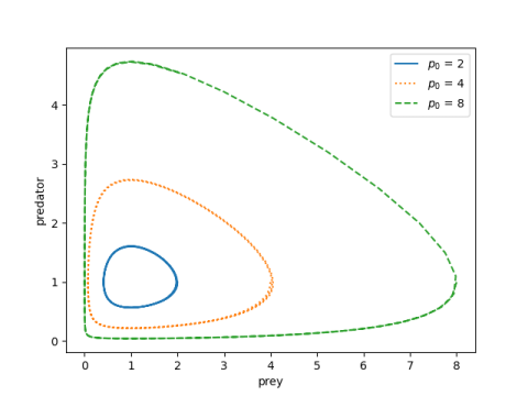
Phase plot

Here is a plot of (x(t), y(t)) showing that the solutions are periodic.

And here's the Python code that made the plot above.

 import matplotlib.pyplot as plt import numpy as np from scipy.integrate import solve_ivp # Lotka-Volterra equations def lv(t, z, a, b): x, y = z return [a*x*(y-1), -b*y*(x-1)] begin, end = 0, 20 t = np.linspace(begin, end, 300) styles = ["-", ":", "--"] prey_init = [2, 4, 8] a = 1.5 b = 1/a for style, p0 in zip(styles, prey_init): sol = solve_ivp(lv, [begin, end], [p0, 1], t_eval=t, args=(a, b)) plt.plot(sol.y[0], sol.y[1], style) plt.xlabel("prey") plt.ylabel("preditor") plt.legend([f"$p_0$ = {p0}" for p0 in prey_init]) 

Note that the derivative of x is zero when y = 1. Since our initial condition sets y(0) = 1, we're specifying the maximum value of x. (If our initial values of x were less than 1, we'd be specifying the minimum of x.)

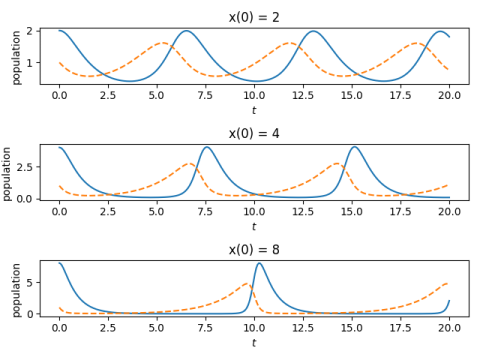
Time plot

The components x and y have the same period, and that period depends on a and b, and on the initial conditions. The plot below shows how the period increases with x(0), which as we noted above is the maximum value of x.

And here's the code that made the plot.

 fig, ax = plt.subplots(3, 1) for i in range(3): sol = solve_ivp(lv, [begin, end], [prey_init[i], 1], t_eval=t, args=(a, b)) ax[i].plot(t, sol.y[0], "-") ax[i].plot(t, sol.y[1], "--") ax[i].set_xlabel("$t$") ax[i].set_ylabel("population") ax[i].set_title(f"x(0) = {prey_init[i]}") plt.tight_layout()

Finding the period

In [1] the author develops a way to compute the period of the system as a function of its parameters without solving the differential equations.

First, calculate an invariant h of the system:

Since this is an invariant we can evaluate it anywhere, so we evaluate it at the initial conditions.

Then the period only depends on a and h. (Recall we said we can scale the equations so that ab = 1, so a and b are not independent parameters.)

If h is not too large, we can compute the approximate period using an asymptotic series.

where = (a + b)/2 = (a^2 + 1)/2a.

We use this to find the periods for the example above.

 def find_h(a, x0, y0): b = 1/a return b*(x0 - np.log(x0) - 1) + a*(y0 - np.log(y0) - 1) def P(h, a): sigma = 0.5*(a + 1/a) s = 1 + sigma*h/6 + sigma**2*h**2/144 return 2*np.pi*s print([P(find_h(1.5, p0, 1), 1.5) for p0 in [2, 4, 8]])

This predicts periods of roughly 6.5, 7.5, and 10.5, which is what we see in the plot above.

When h is larger, the period can be calculated by numerically evaluating an integral given in [1].

Related posts

• Finding the period of Van der Pol oscillations
• The Brusselator
• Lorenz system

[1] Jorg Waldvogel. The Period in the Volterra-Lotka Predator-Prey Model. SIAM Journal on Numerical Analysis, Dec., 1983, Vol. 20, No. 6, pp. 1264-1272

The post Predator-Prey period first appeared on John D. Cook.