QEF13 – Quantum supply and demand

The neoclassical X-shaped supply and demand diagram is featured in every introductory textbook, is the basis for mathematical models of the economy, and has shaped our view of the economy for over a century, but as critics have pointed out many times it has a few basic problems (see Economyths for a summary).

It assumes static equilibrium so there is no dynamics. Supply and demand are assumed to be independent, when we know they are often coupled. And finally, there is no empirical validation for the diagram. For example demand curves involve hypothetical transactions which we can never observe. We also know that prices are not drawn to a stable equilibrium, but are subject to complex dynamics.

The quantum version starts by observing that supply and demand are two sides of the same coin, so what counts is the degree of imbalance - if both increase at the same time it has no effect on price (at least to first order). Modelling potential transactions with a quantum oscillator then leads to a version of the square-root formula derived for price impact in QEF12.

To start with a simple illustration, consider a scenario where there is one seller and one buyer for some perishable item such as a loaf of bread. The seller wants to sell one unit per day, and the buyer wants to buy one unit per day, so the system is balanced. We can model this using an oscillator in the ground state, where the wave function rotates around the real axis with a frequency of once per day, and the squared amplitude representing the joint propensity function is a normal curve.

Suppose now that another buyer enters the picture. The expected transaction rate will therefore double, and the supplier may not be able to keep up. In order to restore the original frequency, the required price increase from the formula is x=2 where measures the degree of price flexibility. Making this change requires energy E=2. As mentioned in QEF09 this is the base quantum of energy which allows for the possibility of a transaction between two people. The energy added by increasing the frequency is therefore balanced by the energy spent in increasing the price.

Left panel shows the probability distribution for the oscillator in the ground state. Adding an additional buyer shifts the oscillator to the right (as indicated by arrow). Right panel depicts the complex wave function rotating around the real axis.

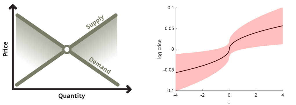
In the general case, define the imbalance to be = (Nb - Na )/min(Na,Nb ) where Na is the number of sellers and Nb is the number of buyers. As with the price impact result from QEF12, we then get a change in log price of x=Y|| where Y=2 and the sign depends on the sign of . This formula is shown in the right panel of the figure below.

Left panel shows the neoclassical supply and demand diagram. Source: Instant Economics. Right panel shows the quantum version with the uncertainty parameter set to =0.02. Change in log price has a square-root dependency on the demand/supply imbalance . The shaded area, representing price uncertainty, shows one standard deviation.

Another feature of the quantum oscillator model is that volatility is a function of the energy level, so if the energy state is En then the volatility will be n=(2n+1)=(||+1). It follows that observed volatility is not a constant, as usually assumed in finance, but varies depending on energy level. The uncertainty therefore increases with the degree of market imbalance, which is consistent with the large fluctuations seen during times of market stress.

If we assume the model is perturbed at each step by an amount x= as in QEF12, then the energy of the system follows a Poisson distribution with average given by =1/4. This modifies the multiplicative constant for the price impact formula slightly to Y=(4/3) which is in the correct range.

To summarise:

• The quantum model treats supply and demand, not as fixed or independent, but as two coupled aspects of a single dynamic process

• Transactions are inherently probabilistic - the uncertainty parameter is not an external noise term or addition, but is integral to the formula

• The model responds dynamically to perturbations, and produces non-Gaussian statistics due to changing volatility

• The model predicts (or postdicts) the square-root law of price impact, including a value for the multiplicative constant

For details, see the SSRN discussion paper Quantum impact and the supply-demand curve.

Previous: QEF12 - A quantum oscillator model of stockmarkets

Playlist: Quantum Economics and Finance