The numerical range ellipse
Let A be an n * n complex matrix. The numerical range of A is the image of x*Ax over the unit sphere. That is, the numerical range of A is the set W(A) in defined by
W(A) = {x*Ax | x n and ||x|| = 1}
where x* is the conjugate transpose of the column vector x.
The product of a row vector and a column vector is a scalar, so W(A) is a subset of the complex plane .
When A is a 2 * 2 matrix, W(A) is an ellipse, and the two foci are the eigenvalues of A.
Denote the two eigenvalues by 1 and 2 . Denote the major and minor axes of the ellipse by a and b respectively. Then
b^2 = tr(A*A) - |1|^2 - |2|^2.
where tr is the trace operator. This is the elliptical range theorem [1]. The theorem doesn't state the major axis a explicitly, but it can be found from the two foci and the minor axis b.
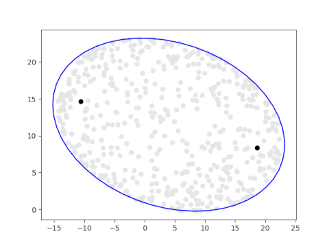
DemonstrationWe will create a visualization the numerical range of a matrix directly from the definition, generating xs at random and plotting x*Ax. Then we draw the ellipse described in the elliptical range theorem and see that it forms the boundary of the random points.
The following code plots 500 random points in the numerical range of a matrix formed from the numbers in today's date. The eigenvalues are plotted in black.
import numpy as npfrom scipy.stats import normimport matplotlib.pyplot as pltA = np.array([[8, 16], [20, 23j]])for _ in range(5000): v = norm(0, 1).rvs(size=4) v /= np.linalg.norm(v) x = np.array([v[0] + 1j*v[1], v[2] + 1j*v[3]]) z = np.conj(x).dot(A.dot(x)) plt.plot(z.real, z.imag, 'o', color='0.9')eigenvalues, eigenvectors = np.linalg.eig(A) plt.plot(eigenvalues[0].real, eigenvalues[0].imag, 'ko')plt.plot(eigenvalues[1].real, eigenvalues[1].imag, 'ko')
The following code draws the ellipse guaranteed by the elliptical range theorem.
A_star_A = np.dot(np.conj(A).T, A)b = (np.trace(A_star_A) - abs(eigenvalues[0])**2 - abs(eigenvalues[1])**2)**0.5c = 0.5*abs(eigenvalues[0] - eigenvalues[1])a = (2/3)*(2*(2*b**2/4 + c**2)**0.5 + c)t = np.linspace(0, np.pi*2)z = a*np.cos(t)/2 + 1j*b*np.sin(t)/2u = (eigenvalues[1] - eigenvalues[0])/2u /= np.linalg.norm(u)m = eigenvalues.mean()z = z*u + mplt.plot(z.real, z.imag, 'b-')
Here is the result.
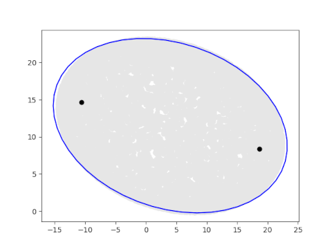
Here is the result of running the same code with 10,000 random points.
[1] Ulrich Daepp, Pamela Gorkin, Andrew Shaffer, and Karl Voss. Finding Ellipses: What Blaschke Products, Poncelet's Theorem, and the Numerical Range Know about Each Other. MAA Press 2018.
The post The numerical range ellipse first appeared on John D. Cook.