Period of a nonlinear pendulum

The term nonlinear pendulum" is analogous to a retronym, a new name for an old thing to distinguish it from a new variation. For example, once upon a time a guitar was just a guitar. Now such a guitar is called an acoustic guitar to distinguish it from an electric guitar. Similarly, analog signal processing is a retronym to distinguish what was once the only kind of signal processing from the new arrival, digital signal processing.

The equation of motion for a pendulum is nonlinear. If the initial angle of displacement is sufficiently small, the linearized form of the equation is adequate for most applications. This linearized approximation is better known than the more accurate original equation, and so the un-linearized equation is known as the nonlinear pendulum equation.

The (nonlinear) equation of motion for a pendulum is the differential equation

where g is the acceleration due to gravity and is the length of the pendulum. For small initial displacement ₀ the linear approximation

works well. The smaller ₀ is the more accurate the linear approximation is.

Linear and nonlinear period

The period of a pendulum obtained by solving the linearized equation is

The solution to the nonlinear pendulum equation is also periodic, though the solution is a combination of Jacobi functions rather than a combination of trig functions. The difference between the two solutions is small when ₀ is small, but becomes more significant as ₀ increases.

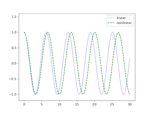
The difference in the periods is more evident than the difference in shape for the two waves. The period of the nonlinear solution is longer than that of the linearized solution. Here's a plot of the solutions to the linear and nonlinear equations, with = g and ₀ = 1.

The period for the nonlinear pendulum is given by

where f is an increasing function, equal to 1 at = 0.

The exact form of f involves special functions, and so there is naturally a lot of interest in approximations to f. The exact value is given by

where K is the complete elliptic integral of the first kind" and AGM is the arithmetic-geometric mean.

The AGM of two numbers is found by taking their ordinary (arithmetic) mean and geometric mean, then repeating the process. This process converges very rapidly, and so doing one step of the iteration gives a good approximation. If that's not good enough, doing two steps gives an even better approximation, and so on. In fact, a common approximation for f() is to do half a step, taking the geometric mean of 1 and cos(/2), i.e.

To see how accurate this approximation is, let's plot the exact and approximate values of f.

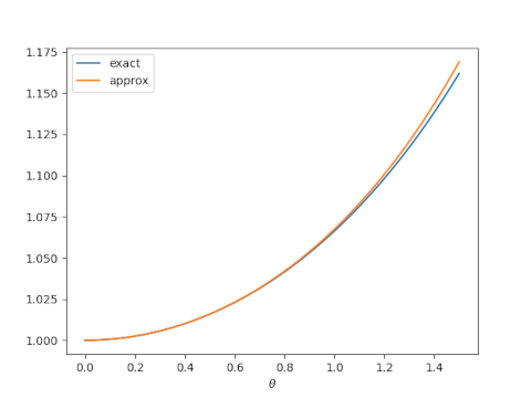
The two curves can hardly be distinguished visually, so let's look at a plot of their difference.

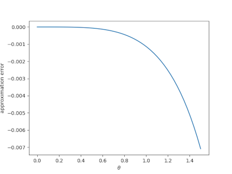
Here's the code that produced the two plots above.

from scipy.special import ellipkfrom numpy import sin, cos, pi, linspaceimport matplotlib.pyplot as pltdef exact(): return 2*ellipk(sin(/2)**2)/pidef approx(): return cos(/2)**-0.5t = linspace(0, 1.5)plt.plot(t, exact(t))plt.plot(t, approx(t))plt.xlabel(r"$\theta$")plt.legend(["exact", "approx"])plt.savefig("nonlinear_pendulum1.png")plt.close()plt.plot(t, exact(t) - approx(t))plt.xlabel(r"$\theta$")plt.ylabel("approximation error")plt.savefig("nonlinear_pendulum2.png")

NB: There are two conventions for defining the complete elliptic integral of the first kind. SciPy uses a convention for K that requires us to square the argument.

Driven oscillations

The differences between the linearized and nonlinear equation become more apparent when there is a forcing function, i.e. when the right-hand side of the differential equations is not zero. Here are the solutions when the forcing function is cos(2t).

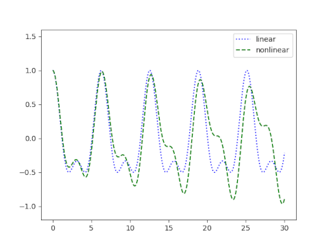
Now the solutions not only differ in their period, the shapes of the solutions are substantially different. The linear solutions are well-behaved but the nonlinear solutions can be chaotic with sensitive dependence on initial conditions. This remains true if a damping term is added.

Related posts

• Kinds of elliptic integrals
• Period of Van der Pol oscillators
• The magic AGM box
• Damped, driven (linear) oscillations

The post Period of a nonlinear pendulum first appeared on John D. Cook.